Available Volume
The Available Volume method, as the name suggests, allows us to reconstruct the maximum volume which can be sampled by each dye attached to a specific residue on a macromolecule; and to calculate the transfer efficiency distribution between two dyes. It is done by replacing the dye with a simple segmented linker and a sphere with a radius equal to one of the three dye headgroup dimensions. The volume accessible to each dye is reconstructed by drawing a number of positions and choosing only those which do not overlap with the host molecule. The most important assumption of this method is that all possible positions within the volume are equally probable. This method does not provide any information about the orientation factor, so we can use it only within the limits of the isotropic approximation. The algorithm for calculating the Available Volume was adapted and modified from the original one published by Sindbert et al. (J. Am. Chem. Soc., 2011, 133, 2463–2480)
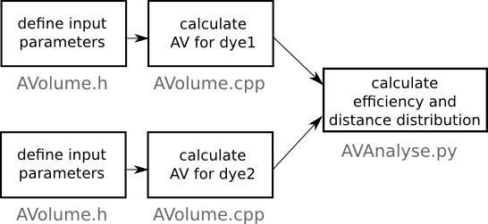
How to use?
Compiling the program
- Download and unpack the source of AV program (here).
- All parameters of the system and dyes should be written into a AVolume.h file.
- The source file (AVolume.cpp) and pseudorandom number generator (random_number.cpp) has to be compiled together using any C++ compiler, for example:
g++ AVolume.cpp random_number.cpp -o program.x
- The program needs to be compiled every time parameters in AVolume.h are changed.
- The recommended use of the program is:
./program.x
- The program will produce an output files (.dat and .pdb) with the names defined in AVolume.h.
Visualising the available volume
- The volume available to the dye can be visualised through the output pdb file.
- For example in VMD, load the pdb file and represent with the QuickSurf method or as VdW spheres.
- The positions stored in the pdb represent the middle of the headgroup.
- The volume available for each headgroup radius can be separately visualiused as each has a different resname (VR1, VR2, VR3)
FRET analysis
- Compile and run the main program as above for each dye (you should now have two .dat files).
- You need to have python installed with numpy, matplotlib & matplotlib-tk
- Run the AVanalyse.py script to
calculate the distance and
FRET efficiency distribution for the pair
of dyes. The analysis script is divided
into several blocks which can be run
seperately. However, to run some of them
it is necessary to previously run the one
before.
To run the script, just change parameters inside it describing the .dat file names and the headgroup sizes (to run selected blocks, just set the value of their indicator from 0 to 1) and type:
python AVAnalyse.py
- Running may take some time (~25 mins for the example files)
- It will produce the output file, for example histogram_AF488_AF594s.dat, which contain the histograms of the distance and FRET efficiency distribution.
- The raw output assumes each photon is detected separately. In reality, most experimental data is the average of multiple photons. To see how this changes the histograms you can run the script BurstAvg.py by setting the number of photons to average in each burst at the top of the script and running:
python BurstAvg.py