The Rotamer library method first determines the most probable dye conformations in the absence of the macromolecule and then superimposes thes upon the macromolecular scaffold. It thus can provide information about the orientation factor as well as about the existence of favourable dyes conformations. This method is succesfully used in the analysis of spin labels in electron paramagnetic studies but has not previously been adapted to use in FRET. Using preliminary molecular dynamics simulations, we identify several likely conformations of the dye, which are defined by the set of dihedral angles. Each set of dihedrals represents a single rotamer, whose weight represents the probability of the dye adopting that conformation.

How to use?

• All scripts can be download here. You need also to install catdcd and some pythons libraries: numpy, matplotlib, and MDAnalysis.

Pre-calculated libraries

Here we provide pre-calculated libraries for several common fluorescence dyes. The rotamer libraries are stored in the form of dcd files that can easily be visualised in biomolecular graphics programs.

• AlexaFluor 488 (maleimide derivative attached to the CYS residue) dcd, pdb, dat
• AlexaFluor 594 (maleimide derivative attached to the CYS residue) dcd, pdb, dat
• AlexaFluor 594 (succinimide ester attached to the GLY residue) dcd, pdb, dat
• Cyanine Cy3 (maleimide derivative attached to the CYS residue) dcd, pdb, dat
• Cyanine Cy5 (maleimide derivative attached to the CYS residue) dcd, pdb, dat

Building new rotomer libraries

• This requires you to have python, numpy, scipy, MDAnalysisTools and catdcd installed
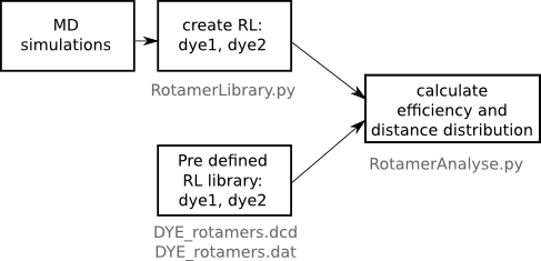
• To build a rotamer library you need to run a preliminary set of MD simulations of the free dyes in water box. In our simulations the dye was attached to either a fixed CYS or GLY residue. From these simulations you need the .pdb and .dcd files
• These simulations can be transformed into RL library used our python script RotamerLibrary.py.
• To run this first open set the name of the pdb and dcd file from your preliminary MD simulation (eg AF488.pdb, AF488.dcd) and the number of flexible dihedrals in the molecule. Then, you have to specify atom numbers related to each of these dihedrals (this part may be a bit time consuming, especially if the dye linker is long). You can also select which block of the program to run, but note that some blocks require previous blocks to have already been completed.
• Run the script
  
  python RotamerLibrary.py
  
  
• Creating the libraries can take some time, depending on the size of the dcd file. Expect anywhere from 20 mins for 1000 frames to 20 hours for 50,000 frames when running on 1 CPU.
• The rotamer libraries are stored in the form of a dcd file of dye without water (DYE_rotamers.dcd) that can easily be visualised in biomolecular graphics programs, along with a file containing the specific diehedral angles and weights of each rotamer (DYE_rotamers.dat). Note, that if you are building your library using any dcd file, you have to provide consistent pdb. The RotamerLibrary.py produces dcd file with dye conformations only, without water, so the pdb file using in further calculations also need to be without water.
• Feel free to send us any rotamer libraries you create so that we can add them to this page to be used by other researchers.

FRET Analysis

• Once the rotamer libraries are ready and the macromolecular system is chosen, the analysis script RotamerAnalyse.py should be run to calculate the distance, orientation and FRET efficiency distribution for the pair of dyes on the macromolecule. The analysis script is divided into several blocks which can be run seperately.
  
• Before running the script, first change parameters inside it describing the names of the rotomer library files, the number of atoms in each dye, the R0 value, average atom size (for overlaping condition) and proper selections for atoms in system (to run selected blocks, just set the value of their indicator from 0 to 1).
• Run by typing:
  
  python RotamerAnalyse.py
  
  It will produce the output file, for example histogram_RL.dat, which contain the histograms of the distance and FRET efficiency distribution.
  
  
• Runing the script can take some time, depending on the size of the libraries. For the examplary files it is 1.5 hours when running on 1 CPU.
• The raw output assumes each photon is detected separately. In reality, most experimental data is the average of multiple photons. To see how this changes the histograms you can run the script BurstAvg.py by setting the number of photons to average in each burst at the top of the script and running:
  
  python BurstAvg.py